Grasshopper Solution Exception Could Not Find Node
Structural analysis with Karamba
![]()
As we discussed previously, metrics are a crucial aspect of the generative design framework because they allow an optimization algorithm to automatically evaluate the relative performance of different design options in a design space and use that information to target better designs. Although the metrics you choose depend on the design problem you are trying to solve, computer simulation techniques provide a range of useful strategies for predicting the performance of a design object in the physical world.
One of the most popular of these methods is static structural simulation through finite element analysis (FEA). This type of simulation represents physical objects as a collection of discrete components or 'elements'. These elements can be represented by 1-dimensional (line), 2-dimensional (planar mesh face), or 3-dimensional (tetrahedron) geometries. The FEA simulation uses these elements to calculate how forces originating from some load applied to the object distribute themselves throughout the object's form. Based on this calculation and the material properties of each element, it can then predict how much the object will move under load, and the stress that each element will experience as a result.
Assuming that the object does not undergo substantial movement or deformation under the given load, this simulation can be calculated 'statically', in other words based on a single calculation. This means that the calculation can be done much faster than with other more complex 'dynamic' simulations such as computational fluid dynamics (CFD) or dynamic structural analysis, which rely on many calculations executed repeatedly over many time steps. The speed of the analysis makes it particularly useful for generative design, where depending on the complexity of the design space we may need to generate and evaluate many thousands of design iterations before finding the optimal solutions.
Grasshopper Karamba
Another advantage of FEA simulation is that it can be easily integrated into our Grasshopper-based generative design workflow using the Karamba plugin. The full version of Karamba requires a license, but there is also a free version that provides basic functionality while allowing unlimited use. You can download the latest version of the plugin here, just make sure that you download the version that matches the version of Rhino you are using (32 or 64 bit). For this demo I will be using Karamba version 1.2.2 for Rhino 5 64-bit. You can find archived installation packages for this version here.
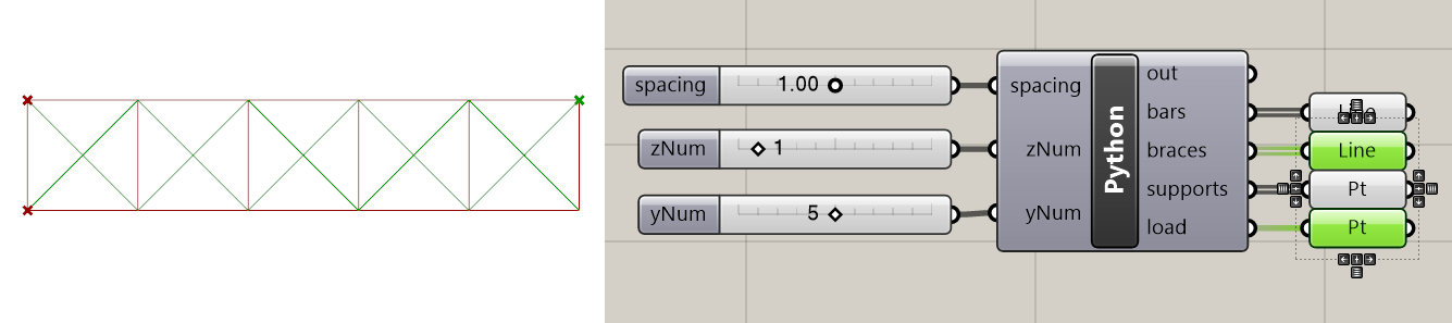
Let's go through the process of running a basic structural analysis in Karamba using a simple example of a cantilevering truss. You can follow along with the process using your own example, or you can download this grasshopper file which contains a Python node for generating a simple truss. The node takes inputs for the size and number of modules in the truss and generates line geometry for the main structural elements and cross-braces as well as point geometry for the areas where the structure is supported and where the load is applied. If you get stuck along the way you can also download the final working version of the definition here.
Before we begin setting up the analysis model, you should consider the base units of your Rhino file. When you install Karamba you have to specify which units you want it to work with, which can be either SI (metric) or imperial units. If you choose to work with SI units Karamba will always assume that your model is in meters. This will cause problems if your Rhino file is using a different base unit such as feet or millimeters, so make sure you convert your model to meters (or feet if using imperial) before starting to work with Karamba.
Assembling the model
To perform structural analysis in Karamba, you must first convert your Grasshopper or Rhino geometry to a simulation model. This is done using the Assemble node in the Karamba library, which you can find in the 'Model' area of the Karamba toolbar.
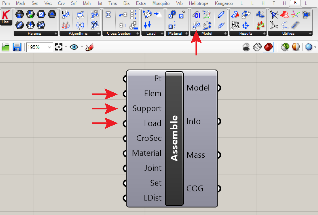
The Assemble node collects all the necessary information about a structural analysis problem and produces a model that is ready for analysis. At a minimum, the model requires the specification of one or more elements (these can be 1-dimensional beam elements based on line segments, or 2-dimensional shell elements based on meshes), one or more points where the model is rigidly supported, and one or more loading conditions which apply force to the model. Karamba provides special nodes for specifying each of these elements based on Grasshopper geometry. The required inputs to the Assemble node are shown with red arrows in the image above. The other inputs allow you to specify additional features and options for the analysis, but since they all come with default settings their specification is not strictly required for running the simulation.
Creating elements
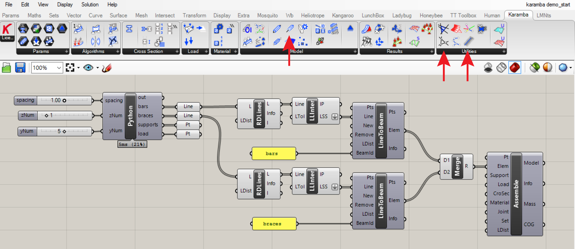
In our example, the elements will be the line segments of the truss. We can convert lines in Grasshopper to Karamba beam elements using the LineToBeam node found in the 'Model' area of the Karamba toolbar. This node takes in line geometry from Grasshopper and converts it to a series of beam elements which can then be input into the Assemble node.
In addition to 1-dimensional beam elements based on line geometry Karamba also supports 2-dimensional shell elements based on mesh geometry. You can easily combine beam and shell geometry within a single analysis model as long as the lines and meshes connect at the same vertices. For example, you can simulate a building's structure by using beam elements for columns and shell elements for floors. For a good example of analyzing shell elements based on mesh geometry you can look at this example.
Karamba provides a set of useful nodes for pre-processing line geometry before converting it to beams:
- The
RDLinesnode removes duplicate line geometry. Duplicate lines are difficult to see in the model but will effect the results of your analysis so it is a good idea to always pass your line geometry through this node before passing it to theLineToBeamnode. - The
LLInternode solves line-to-line intersections and outputs the results of splitting each line with every other line in a set. This is also good practice before making beam elements because by default if two lines cross they will slip past each other instead of connecting, which is typically not what you want. The output of this node will be in data tree format so make sure you flatten it before passing it to theLineToBeamnode.
In our case we have two separate sets of lines we want to use as beam elements (the 'bars' and 'braces'). We will create two separate sets of beams from them and will assign them unique BeamID's so that we can later give them different material and cross sectional properties. The BeamID's can be any combination of letters and numbers, but they cannot be single integers. We will first merge the two sets of beam elements produced by the two LineToBeam nodes using a Merge node before plugging them into the 'Elem' input of the Assemble node. Make sure that all the elements come into the Assemble node as a single flat list. Otherwise if you input a data tree the node will actually create separate models for each branch of the tree.
Specifying supports
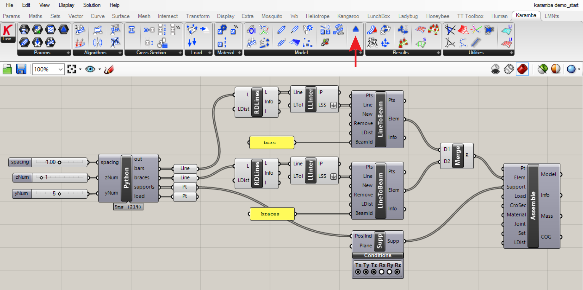
Once we've created the elements of the analysis model, we need to specify how the model is supported. We can do this using the Support component found in the 'Model' area of the Karamba toolbar. This component takes in a series of points from Grasshopper and converts them to fixed points in the model. In order to work correctly the points specified should already exist in the model as either the endpoints of beam elements or the vertices of shell meshes. If Karamba can't find the points in the model the Assemble node will produce an error similar to this one:
Could not find node at (X/Y/Z) where support number _ is attached The six radio buttons inside the Support node allow you to specify how the support points are fixed based on the six degrees of translational and rotational freedom. How these are specified depends on your problem setup, but the constraints should be enough such that your model does not move freely in space. If in doubt you can simply enable all six constraints to rigidly fix the support nodes in all directions. Once we have specified the support condition we can connect the output of the Support node to the 'Support' input of the Assemble node.
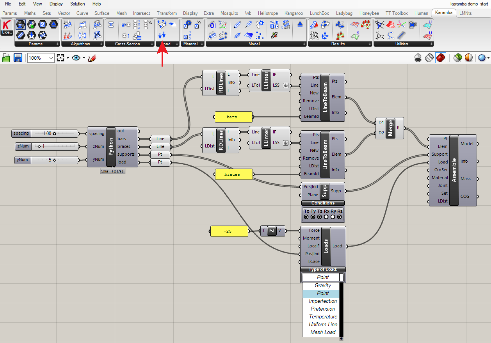
Specifying loads
The final thing we need to do to have a valid structural simulation model is to specify one or more loads that are applied to the model. We can do this using the Loads component found in the 'Load' area of the Karamba toolbar. This is a multi-use component which allows us to specify a number of different types of loads for the model. You can select the type of load using the drop-down menu at the bottom of the node. Once you select a load type the inputs of the node will change based on the information required for each load case. The simplest type of load is 'Gravity' which does not require any additional inputs and calculates the force due to gravity applied to each element in the model
In our case we will apply a 'Point' load to the end of the cantilevering truss. Similar to the Support node, the Point load requires one or more points from Grasshopper which it will find as nodes in the model and apply the loads to. Just as before, these points should already exist in the model as either end points of beam elements of vertices of shell meshes. The Point load also requires you to specify the magnitude and direction of the load using a vector from grasshopper. In this case we will specify a vector of magnitude '25' pointing down in the z-direction. If using SI units the loads are specified in Kilonewtons (kN). Once we have specified the load condition we can connect the output of the Loads node to the 'Load' input of the Assemble node.
Specifying materials and cross-sectional properties
The final thing we may want to do before running our analysis is to specify the shape of our beam elements, and the materials they are made out of. These options have default settings in Karamba so their specification is not strictly necessary to run the analysis. However, they will have a big effect on the results so should be specified based on your design.
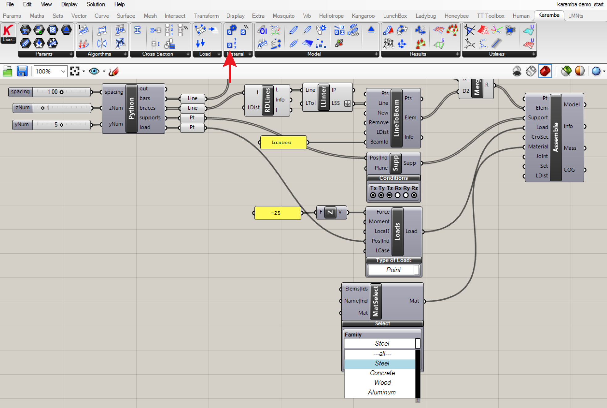
Material properties can be specified using the MatSelect node found in the 'Material' area of the Karamba toolbar. You can select a predefined material from Karamba's library by using the drop-down menus at the bottom of the node. You can also use the MatProps node to specify your own material properties. If you want to assign different material properties to different elements in your model you can use the 'Elems|Ids' input of the node to specify the ID name of the elements that the material should be applied to. In this case we will leave this input blank to apply the basic 'Steel' material to every element of the model. Once we have specified the material properties we can connect the output of the MatSelect node to the 'Material' input of the Assemble node.
The shape of the beam elements is specified according to the beam's cross-section. Remember that the beam elements are 1-dimensional objects based on lines. In order to tell Karamba how the beams perform structurally we need to specify their shape in the other two dimensions. You can think of cross sections astwo dimensional shapes which are 'extruded' along the length of the beam.
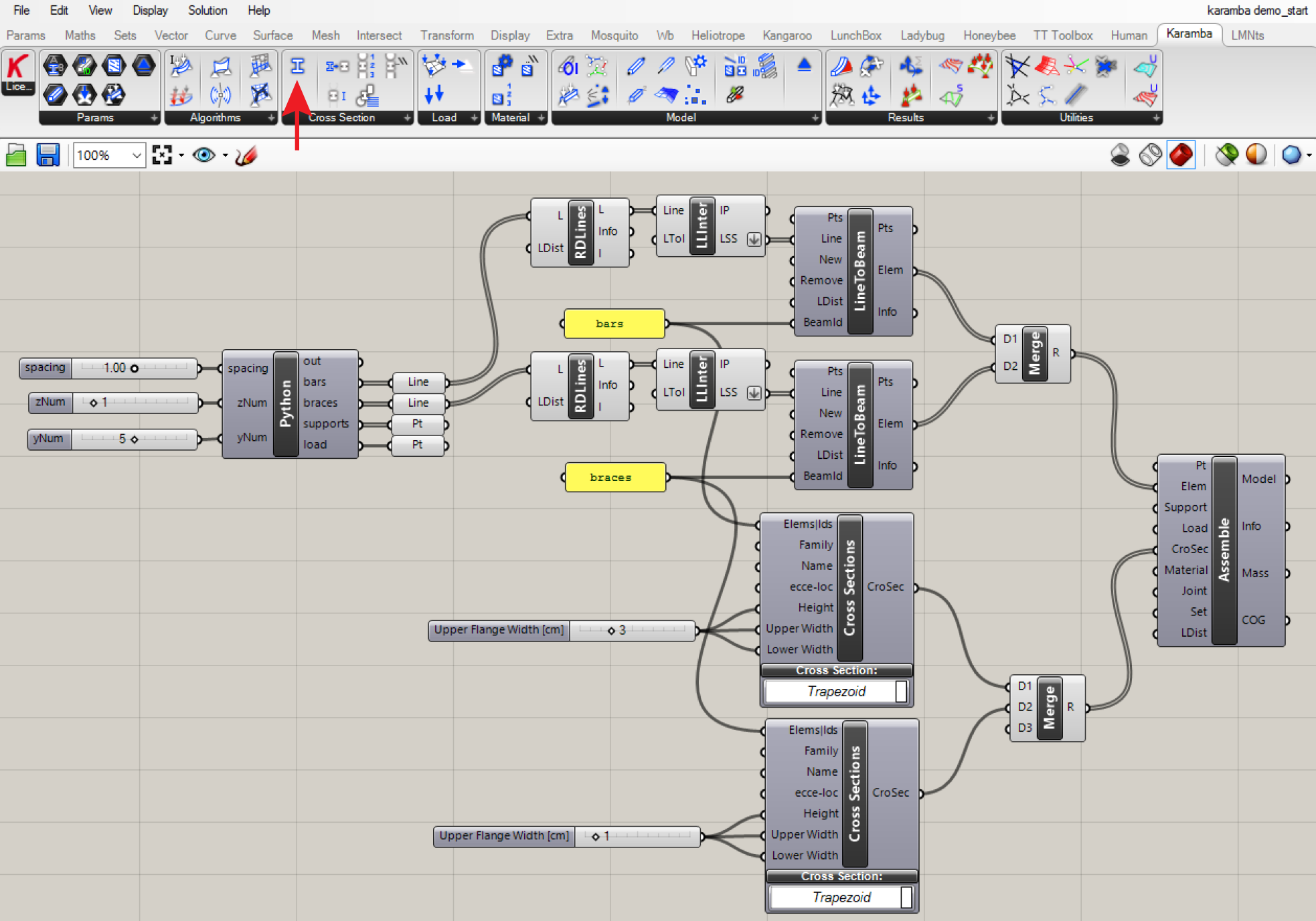
The cross-section properties of beams can be specified using the Cross Sections node found in the 'Cross Section' area of the Karamba toolbar. You can select one of Karamba's predefined cross-section types by using the drop-down menus at the bottom of the node. Once you select a cross-section type the inputs of the nodes will change based on the information required to define each type of cross-section.
In our case we will use the 'Trapezoid' section which defines a solid quadrilateral section based on dimensions for the height and the two bases of the trapezoid. To define a square cross-section we simply use the same dimension for all three parameters. We will create two different cross-sections for our two types of beam elements — a larger one for the main structural elements and a smaller one for the cross braces. To tell Karamba which cross-sections to apply to which elements we will connect the BeamID's we specified previously to the 'Elems|Ids' inputs of the two Cross Section nodes. Once we have specified the two cross section types we will merge them using a Merge node before inputting them into the 'CroSec' input of the Assemble node.
Calculating the model
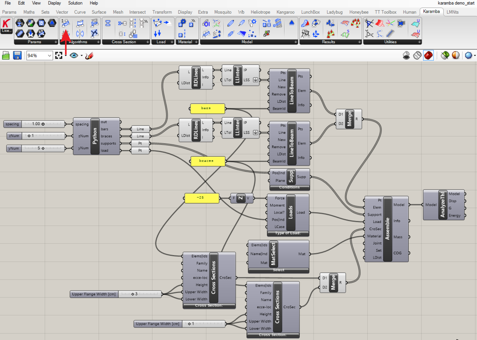
Once our model is specified and assembled, we can perform the structural calculation by choosing an analysis component from the 'Algorithms' area of the Karamba toolbar and connecting it to the 'Model' output of the Assemble node. Karamba includes a number of analysis components for performing different types of structural calculations. The most important are :
- the
AnalyzeThlcomponent for analyzing models undergoing small deflections - the
LaDeformcomponent for analyzing models undergoing large deflections
In building-scale or structural engineering applications such as truss design we typically deal with very small structural deflections which can be easily simulated all at once using a static analysis. For these static cases you can use the AnalyzeThl node. In some applications, however, you may want to analyze structures which undergo large deflections (for example finding the equilibrium shape of a hanging structure). To be accurate such structures need to be calculated dynamically over a series of time steps using the LaDeform node.
In our case we are dealing with a fairly rigid truss structure so we can use the AnalyzeThl component to perform the analysis. Let's place this node on the canvas and connect it to the 'Model' output of the Assemble node. If the model has been specified correctly the node will turn grey and won't generate any warnings or errors. The most common reason for the analysis node to generate errors is if the model is not properly fixed with the supports and can move freely in space.
Visualizing results
Once the model has been calculated we can visualize the results of the structural analysis in Grasshopper. Karamba provides three main 'View' nodes for visualizing the analysis results:
-
Model View— allows you to label various components of the model and visualize the shape of the model under deformation. -
Beam View— allows you to visualize performance data as colors directly on the model's beam elements. -
Shell View— allows you to visualize performance data as colors directly on the model's shell elements.
All three of these nodes are found in the 'Results' area of the Karamba toolbar. Each of them have a 'Model' input that takes in an analyzed structural model for visualization, as well as a 'Model' output which returns the structural model with the visualization information attached. This allows you to chain together multiple visualization nodes to generate a variety of visualization types.
Let's create a visualization of the deflected truss with structural performance information visualized on the beam elements. To do this we'll first pass the model through a Model View node to create the deflected shape, and then through a Beam View node to visualize the performance of each beam.
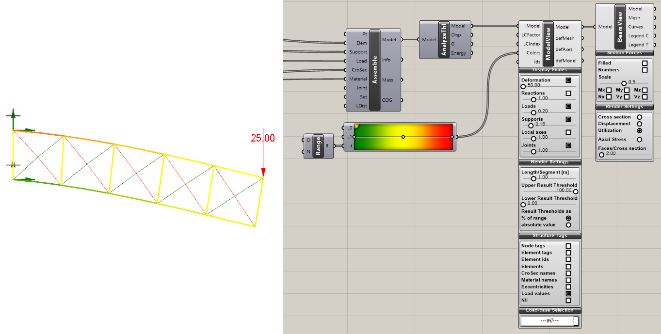
Along with the model, the Model View node can also take in a list of custom colors which it will use for the visualization. The easiest way to create this list of colors is to use a Gradient node combined with a Range input to create a list of colors sampled evenly from a gradient.
The options of the visualization nodes can be seen by clicking on the black heading bars, which will unroll a set of options under each heading. The Model View node has a variety of options for visualizing the deformed shape of the structure as well as the various elements of the model. In this case we will visualize the supports of the model as well as the load vector and value.
The Beam View node allows you to visualize different types of structural data as colors directly on the beam elements. The 'Cross section' option colors the beams differently based on their specified cross section. The 'Displacement' option colors the beams based on the distance they move under loading. The 'Utilization' and 'Axial Stress' options color the beams based on how much stress the beams experience under loading. 'Axial Stress' gives the stress information directly, while 'Utilization' expresses the stress in terms of its percentage of the maximum stress capacity of the material (this is based on the material properties specified for the beam).
Utilization numbers can be used to check whether the elements of the model fit within the margin of safety required by a design. A utilization number higher than 100% means that the element is likely to break under the specified load. In our visualization the utilization of each beam is represented by its color, with yellow beams experiencing the least stress, green beams experiencing a high compression stress (high negative utilization) and red beams experiencing a high tensions stress (high positive utilization).
Extracting metrics
The visualization nodes provide a good way to visually check the performance of the structure under the specified load. However, in order to use this analysis in our generative design workflow we need to be able to extract quantitative measures from the model which the optimization algorithm can use to automatically evaluate each design. Structural analysis typically deals with three main metrics:
- Minimization of the weight or mass of the model. We typically want to design the smallest or lightest structure which achieves the minimum performance required.
- Minimization of the maximum displacement of the model, or the maximum amount that any element of the structure moves under load. While all structures deflect under loading, there are typically design limits for how much the structure can move.
- Minimization of the stress in the elements of the model. The maximum stress that an element can experience is based on the limits of the material and can be presented either as raw stress values or the utilization of the material as described earlier. Typically you want to ensure that the stresses in all elements of the model fall within some chosen safety factor (for example 50%) of the structural limits of the material.
Let's conclude this section be showing how you can extract these metrics from the Karamba model for use in generative design.
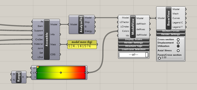
Mass
The model's mass is directly output by the 'Mass' output of the Assemble node. If using SI units the mass will be given in kilograms (kg).
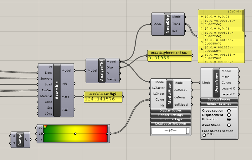
Displacement
The maximum displacement of any node in the model is directly output by the 'Disp' output of the AnalyzeThl component. If you are interested in the displacement of particular nodes you can also use the NodeDisp component found in the 'Results' area of the Karamba toolbar. This component will output both the translation and rotation that each node of the model experiences under loading. If using SI units the displacement values are given in meters (m).
Forces and utilization
Unfortunately the free version of Karamba does not allow you to directly output the stress or utilization of the model's elements. However, you can output the forces that each element experiences under loading. Since stress and utilization are calculated based on the force in each element and its cross sectional and material properties, minimizing the forces experienced by the elements will inherently minimize the stress as well. Although this will not give you any direct information about the structural performance or potential failure of the elements, we can use the force information as a proxy for structural performance during optimization.
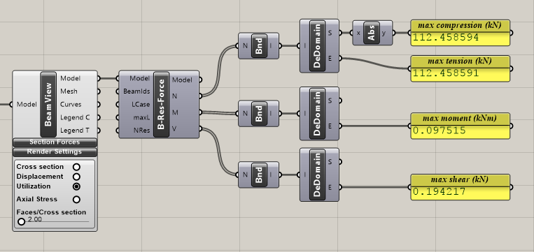
To see the forces in each element of the model we can use the B-Res-Forces node also found in the 'Results' area of the Karamba toolbar. This node will output the axial (N), rotational/moment (M), and shear (V) forces in each element of the model. To calculate the maximum values of each type of force we can use Grasshopper's Bounds component to calculate the range of each set of values, and the DeDomain node to extract the minimum and maximum of the range. Note that axial forces are given as negative values for compressive forces and positive values for tensile forces. Thus, to minimize the overall axial force you would typically minimize both the largest number (highest tensile force) as well as the absolute value of the smallest number (highest compressive force).
Finally, although the free version of Karamba does not allow you to output the stress and utilization values of each element directly, you can extract the highest and lowest values indirectly from the Beam View node. The 'Legend T' output of this node gives you the text portion of the legend generated for the colors of the visualization. Depending on the property you have chosen to visualize, this text will give you the extreme values of the results mapped onto the bars. In our case, the legend tells us the range of utilization values seen in the model.
The trouble is that the legend also contains other pieces of text unrelated to the actual values we're interested in. However, you can easily filter the text and keep only the numerical values we're interested in. To do this using Python you can make a new Python node and enter this code:
            import re            a = []
x.pop(0)            for val in x:
              try:
              a.append( float(re.sub(r'[^\d.-e+]+', '', val)) )
              except ValueError:
              continue
This code will take in a series of values in the 'x' input and produce a series of decimal values in the 'a' output stripped of any non-numeric information. For the code to work make sure that the 'x' input is set to 'List Access'. We can then apply the Abs, Bnd, and DeDomain nodes as before to get the maximum utilization of all elements in the model. As a metric for optimization, we may want to have an objective that minimizes the maximum utilization, or a constraint where this number has to be lower than our chosen safety factor (for example 50).

Hopefully this demo gave you a basic understanding of how you can use the Karamba plugin to perform static structural analysis of a model, visualize the results, and extract a series of metrics to use in the generative design workflow.
Karamba includes many more features which may be useful depending on the nature of your design and the type of analysis you want to do. To see a full list of features you can look through the full Karamba Manual or go through the examples and tutorials on Karamba's website.
Grasshopper Solution Exception Could Not Find Node
Source: https://medium.com/generative-design/structural-analysis-with-karamba-a73b959587c0